Tensorflow: vattenfall

Deep learning to model transient dynamics of hydro Turbine

import pandas as pd
import numpy as np
import matplotlib.pyplot as plt
import seaborn as sns
from pandas.plotting import register_matplotlib_converters
# plt.style.use(['science','no-latex'])
# plt.rcParams["font.family"] = "Times New Roman"
%load_ext autoreload
%autoreload 2

import tensorflow as tf

1, Load the data

#from tensorflow import keras
#from google.colab import drive
#drive.mount('/content/drive')
#df = pd.read_csv('/content/drive/MyDrive/Data/vattenfall_turbine.csv')
#drive.flush_and_unmount()
#print('NB: Unmount the google cloud driver')

df = pd.read_csv(r'E:\FEM\Python\bitbucket\Vattenfall_rnn\vattenfall_turbine.csv')
keys = df.keys().values
feature_keys = keys[np.arange(1,5).tolist() + np.arange(7,10).tolist()]
time_key = keys[0]

plot_cols = feature_keys[0:len(feature_keys):2]
plot_features = df[plot_cols]
#plot_features.index = df[time_key]
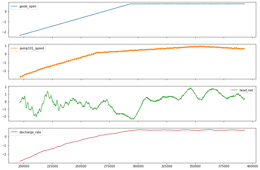
fig1 = plot_features.plot(subplots=True, figsize=(10, 8))
plt.show()

from IPython.display import display, Markdown
#display(Markdown(' <font size="6"><span style="color:blue">**Lets take a close look at the time series.**</span> </font>'))

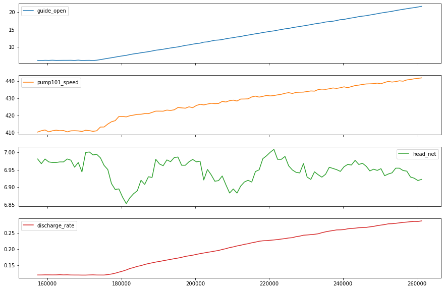
display(Markdown('<span style="color:blue;font-size:50px">**Lets take a close look at the time series.**</span>'))

plot_features = df[plot_cols][int(len(df)/5):int(len(df)/3):1000]
#plot_features.index = df[time_key][:480]
fig2 = plot_features.plot(subplots=True, figsize=(15, 10))

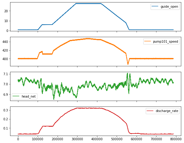
Lets take a close look at the time series.

2, Preprocessing data: normalize, train, validation, test, etc.

2.1, resample the data with low-resolution

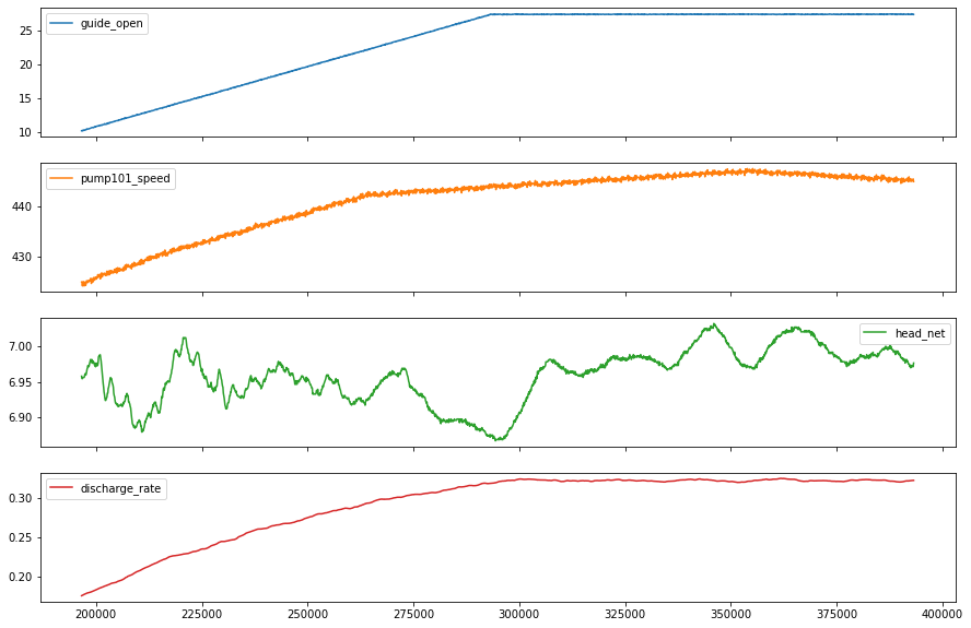
df_train = df[feature_keys[0:7:2]][int(len(df)/4):int(len(df)/2):100]
display(Markdown('<span style="color:red; font-size:30px">**No. of the values in the training dataset is: %d**</span>' %len(df_train)))

# plot the data and check their variations along time
df_train.plot(subplots=True, figsize=(15, 10))
plt.show()
#print('No. of the values in the training dataset is: %d' %len(df_train))

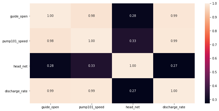
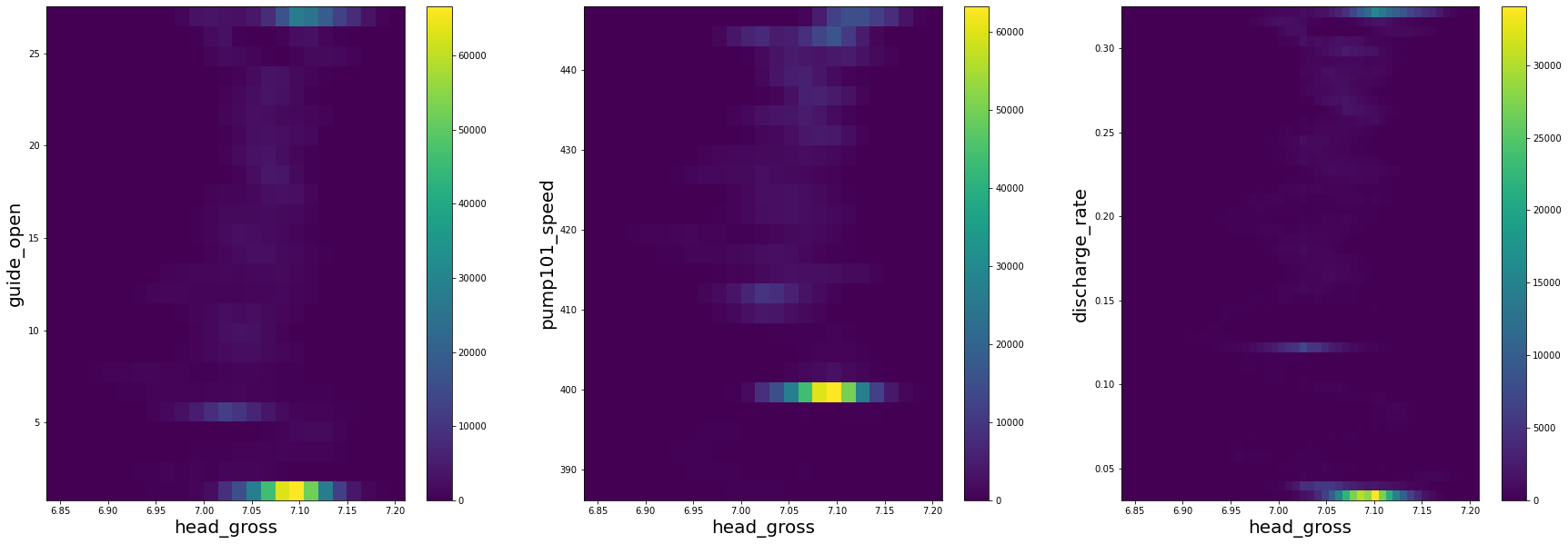
display(Markdown('<span style="color:blue; font-size:20px">**Plot the heatmap for variation of standard deviation**</span>'))
# check he correlation
import seaborn as sns
plt.figure(figsize=(12, 6))
sns.heatmap(df_train.corr(), annot=True, fmt=".2f")
plt.show()

No. of the values in the training dataset is: 1967

Plot the heatmap for variation of standard deviation

from mpl_toolkits.axes_grid1 import make_axes_locatable
from matplotlib import colors, ticker, cm


fig = plt.figure(figsize=(30, 10))
fig.add_subplot(131)
plt.hist2d(df['head_gross'], df['guide_open'], bins=(25, 25))
plt.xlabel('head_gross', size=20)
plt.ylabel('guide_open', size=20)
plt.colorbar()

fig.add_subplot(132)
plt.hist2d(df['head_gross'], df['pump101_speed'], bins=(25, 25))
plt.xlabel('head_gross', size=20)
plt.ylabel('pump101_speed', size=20)
plt.colorbar()

fig.add_subplot(133)
plt.hist2d(df['head_gross'], df['discharge_rate'], bins=(50, 50))
plt.xlabel('head_gross', size=20)
plt.ylabel('discharge_rate', size=20)
plt.colorbar()

<matplotlib.colorbar.Colorbar at 0x28253e14520>

features = df.keys()
features

Index(['time', 'guide_open', 'running_speed', 'pump101_speed', 'pump102_speed',
       'pump101_set', 'pump102_set', 'head_net', 'head_gross',
       'discharge_rate', 'unknow_Hg', 'unknow_Hst', 'unknow_Qt',
       'unknown_Pabs'],
      dtype='object')

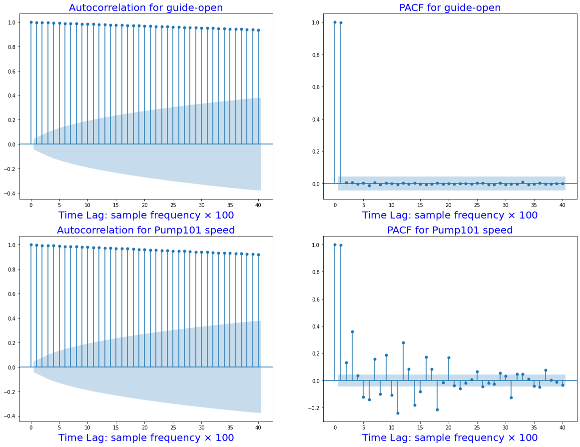
2.2, autocorrelation function (ACF) and (PACF) to check time dependence

def autocorr(x):
    result = np.correlate(x, x, mode='full')
    return result[int(result.size/2):]

acf_open = autocorr(df_train.guide_open)


from statsmodels.graphics.tsaplots import plot_acf
import statsmodels.api as sm

fig, ax = plt.subplots(2,2,figsize=(20,15))
sm.graphics.tsa.plot_acf(df_train.guide_open.squeeze(), lags=40, ax=ax[0,0])
ax[0,0].set_title("Autocorrelation for guide-open", fontsize=20, color='blue')
ax[0,0].set_xlabel(r'Time Lag: sample frequency $\times$ 100', fontsize=20, color='blue')

sm.graphics.tsa.plot_pacf(df_train.guide_open.squeeze(), lags=40, ax=ax[0, 1])
ax[0,1].set_title("PACF for guide-open", fontsize=20, color='blue')
ax[0,1].set_xlabel(r'Time Lag: sample frequency $\times$ 100', fontsize=20, color='blue')

sm.graphics.tsa.plot_acf(df_train.pump101_speed.squeeze(), lags=40, ax=ax[1,0])
ax[1,0].set_title("Autocorrelation for Pump101 speed", fontsize=20, color='blue')
ax[1,0].set_xlabel(r'Time Lag: sample frequency $\times$ 100', fontsize=20, color='blue')

sm.graphics.tsa.plot_pacf(df_train.pump101_speed.squeeze(), lags=40, ax=ax[1,1])
ax[1,1].set_title("PACF for Pump101 speed", fontsize=20, color='blue')
ax[1,1].set_xlabel(r'Time Lag: sample frequency $\times$ 100', fontsize=20, color='blue')
plt.show()

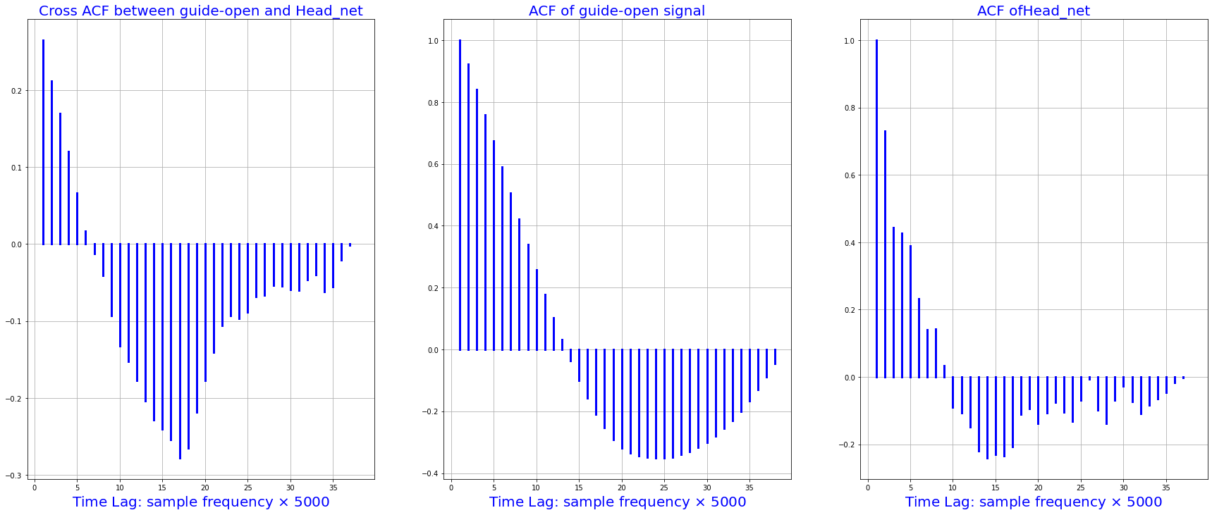
2.3 crossing autocorrelationship for various parameters

# NB: we have resampled the data for the autocorreltion analysis

import statsmodels.tsa.stattools as smt
xacf = smt.ccf(df_train.guide_open.squeeze()[0:1900:50], df_train.head_net.squeeze()[0:1900:50],  adjusted=False)
acf1 = smt.ccf(df_train.guide_open.squeeze()[0:1900:50], df_train.guide_open.squeeze()[0:1900:50],  adjusted=False)
acf2 = smt.ccf(df_train.head_net.squeeze()[0:1900:50], df_train.head_net.squeeze()[0:1900:50],  adjusted=False)


fig, [ax1, ax2, ax3] = plt.subplots(1, 3, sharex=True, figsize=(30,12))
i = 1
for p in xacf:
    x = [i, i]
    ax1.plot([i, i], [0, p],  'b', linewidth=3)
    i= i + 1
ax1.grid(True)
ax1.set_title("Cross ACF between guide-open and Head_net", fontsize=20, color='blue')
ax1.set_xlabel(r'Time Lag: sample frequency $\times$ 5000', fontsize=20, color='blue')


i = 1
for p in acf1:
    x = [i, i]
    ax2.plot([i, i], [0, p],  'b', linewidth=3)
    i= i + 1
ax2.grid(True)
ax2.set_title("ACF of guide-open signal", fontsize=20, color='blue')
ax2.set_xlabel(r'Time Lag: sample frequency $\times$ 5000', fontsize=20, color='blue')

i = 1
for p in acf2:
    x = [i, i]
    ax3.plot([i, i], [0, p],  'b', linewidth=3)
    i= i + 1
ax3.grid(True)
ax3.set_title("ACF ofHead_net", fontsize=20, color='blue')
ax3.set_xlabel(r'Time Lag: sample frequency $\times$ 5000', fontsize=20, color='blue')

plt.show()

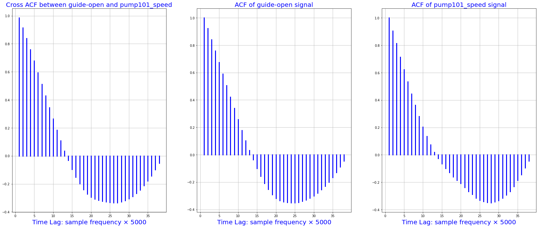
# Autocorrelation between guide_opan and pump101_speed
xacf = smt.ccf(df_train.guide_open.squeeze()[0:1900:50], df_train.pump101_speed.squeeze()[0:1900:50],  adjusted=False)
acf1 = smt.ccf(df_train.guide_open.squeeze()[0:1900:50], df_train.guide_open.squeeze()[0:1900:50],  adjusted=False)
acf2 = smt.ccf(df_train.pump101_speed.squeeze()[0:1900:50], df_train.pump101_speed.squeeze()[0:1900:50],  adjusted=False)


fig, [ax1, ax2, ax3] = plt.subplots(1, 3, sharex=True, figsize=(30,12))
i = 1
for p in xacf:
    x = [i, i]
    ax1.plot([i, i], [0, p],  'b', linewidth=3)
    i= i + 1
ax1.grid(True)
ax1.set_title("Cross ACF between guide-open and pump101_speed", fontsize=20, color='blue')
ax1.set_xlabel(r'Time Lag: sample frequency $\times$ 5000', fontsize=20, color='blue')


i = 1
for p in acf1:
    x = [i, i]
    ax2.plot([i, i], [0, p],  'b', linewidth=3)
    i= i + 1
ax2.grid(True)
ax2.set_title("ACF of guide-open signal", fontsize=20, color='blue')
ax2.set_xlabel(r'Time Lag: sample frequency $\times$ 5000', fontsize=20, color='blue')



i = 1
for p in acf2:
    x = [i, i]
    ax3.plot([i, i], [0, p],  'b', linewidth=3)
    i= i + 1
ax3.grid(True)
ax3.set_title("ACF of pump101_speed signal", fontsize=20, color='blue')
ax3.set_xlabel(r'Time Lag: sample frequency $\times$ 5000', fontsize=20, color='blue')



plt.show()

2.4, normalize the data

# First, we assume all data are used for the training (the time series is not that stationary for the prediction)
df_train_mean = df_train.mean()
df_train_std = df_train.std()
train_df = (df_train-df_train_mean) / df_train_std

fig2 = train_df.plot(subplots=True,figsize=(15,10))

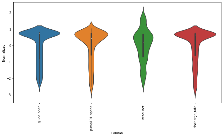
# Second, plot the standand deviation of features within this dataframe
df_std = train_df.melt(var_name='Column', value_name='Normalized')
plt.figure(figsize=(12, 6))
ax = sns.violinplot(x='Column', y='Normalized', data=df_std)
fig3 = ax.set_xticklabels(train_df.keys(), rotation=90)

# tf.convert_to_tensor(new_df)
new_df = train_df.reset_index(drop=True)
target = new_df.pop('guide_open')
#new_df.head()
target.head()
new_df = tf.convert_to_tensor(new_df)

#normalizer = tf.keras.layers.Normalization(axis=-1)
#normalizer.adapt(numeric_features)

feature_keys

array(['guide_open', 'running_speed', 'pump101_speed', 'pump102_speed',
       'head_net', 'head_gross', 'discharge_rate'], dtype=object)

3, Understand the dataset construction and build basic models (treated as independent dataset)

df_train = df[feature_keys][int(len(df)/4):int(len(df)/2):100]

df_train = df_train.reset_index(drop=True)
#df_train.pop('time')
df_train.pop('head_net')
df_target = df_train.pop('head_gross')
df_train.head()

	guide_open	running_speed	pump101_speed	pump102_speed	discharge_rate
0	10.258026	883.147506	424.766713	423.792913	0.175680
1	10.220808	883.147506	424.633645	424.918785	0.176028
2	10.313853	882.934738	423.968301	425.084355	0.176227
3	10.302687	883.041122	424.567110	424.422077	0.176376
4	10.354793	883.041122	424.866515	424.157165	0.176774

# Pre-normalize the features for ML analysis
norm = tf.keras.layers.Normalization(axis=-1)
norm.adapt(df_train)
tf_train = norm(df_train)

# normalize the target (output)
norm_target = tf.keras.layers.Normalization(axis=None)
norm_target.adapt(df_target)
tf_target = norm_target(df_target)

# configure the model
BATCH_SIZE = 500

def get_basic_model():
  model = tf.keras.Sequential([
    norm,
    tf.keras.layers.Dense(50, activation='relu'),
    tf.keras.layers.Dense(50, activation='relu'),
    tf.keras.layers.Dense(1)
  ])

  model.compile(optimizer='adam',
                loss=tf.keras.losses.BinaryCrossentropy(from_logits=True),
                metrics=['accuracy'])
  return model

model = get_basic_model()
model.fit(tf_train, tf_target, epochs=10, batch_size=BATCH_SIZE)

Epoch 1/10
4/4 [==============================] - 1s 4ms/step - loss: 23.7285 - accuracy: 0.0000e+00
Epoch 2/10
4/4 [==============================] - 0s 4ms/step - loss: 0.3162 - accuracy: 0.0000e+00
Epoch 3/10
4/4 [==============================] - 0s 4ms/step - loss: 0.8179 - accuracy: 0.0000e+00
Epoch 4/10
4/4 [==============================] - 0s 4ms/step - loss: 0.2230 - accuracy: 0.0000e+00
Epoch 5/10
4/4 [==============================] - 0s 4ms/step - loss: 0.7362 - accuracy: 0.0000e+00
Epoch 6/10
4/4 [==============================] - 0s 3ms/step - loss: 0.0784 - accuracy: 0.0000e+00
Epoch 7/10
4/4 [==============================] - 0s 4ms/step - loss: 0.2511 - accuracy: 0.0000e+00
Epoch 8/10
4/4 [==============================] - 0s 4ms/step - loss: -0.0369 - accuracy: 0.0000e+00
Epoch 9/10
4/4 [==============================] - 0s 4ms/step - loss: -0.2754 - accuracy: 0.0000e+00
Epoch 10/10
4/4 [==============================] - 0s 4ms/step - loss: -0.2687 - accuracy: 0.0000e+00

<keras.callbacks.History at 0x282a4f19b80>

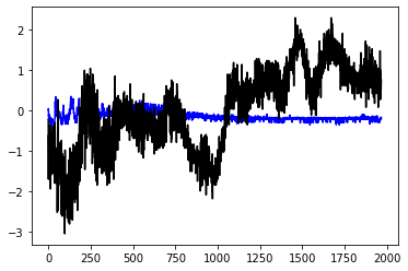
plt.plot(model.predict(df_train),'b')
plt.plot(tf_target,'k')
plt.show()

norm1 = tf.keras.layers.Normalization(axis =-1)
norm1.adapt(df_train)
tf_train = norm1(df_train)

norm2 = tf.keras.layers.Normalization(axis = None)
norm2.adapt(df_target)
tf_target= norm2(df_target)

dataset_df = tf.data.Dataset.from_tensor_slices((tf_train, tf_target))
dataset_batches = dataset_df.shuffle(100).batch(BATCH_SIZE)

model = get_basic_model()
model.fit(dataset_batches, epochs=10)

Epoch 1/10
4/4 [==============================] - 0s 4ms/step - loss: 523.7493 - accuracy: 0.0000e+00
Epoch 2/10
4/4 [==============================] - 0s 5ms/step - loss: 109.0707 - accuracy: 0.0000e+00
Epoch 3/10
4/4 [==============================] - 0s 5ms/step - loss: 55.5138 - accuracy: 0.0000e+00
Epoch 4/10
4/4 [==============================] - 0s 5ms/step - loss: 33.8233 - accuracy: 0.0000e+00
Epoch 5/10
4/4 [==============================] - 0s 4ms/step - loss: 22.7980 - accuracy: 0.0000e+00
Epoch 6/10
4/4 [==============================] - 0s 4ms/step - loss: 16.3655 - accuracy: 0.0000e+00
Epoch 7/10
4/4 [==============================] - 0s 4ms/step - loss: 12.2998 - accuracy: 0.0000e+00
Epoch 8/10
4/4 [==============================] - 0s 4ms/step - loss: 9.7406 - accuracy: 0.0000e+00
Epoch 9/10
4/4 [==============================] - 0s 4ms/step - loss: 7.8712 - accuracy: 0.0000e+00
Epoch 10/10
4/4 [==============================] - 0s 4ms/step - loss: 7.0274 - accuracy: 0.0000e+00

<keras.callbacks.History at 0x282550de250>

3.2, Understand datastructure of the tensorflow package –> formulate rolling windowed dataset –> for model in Section 4

# split the time series of data into train (70%), test (20%) and validation (10%)
#n = len(df_train)
df_train = df[feature_keys]
df_train.pop('head_net')
df_train.pop('discharge_rate')
n = len(df_train)
# start to divide them
train_df = df_train[0:int(n*0.7)]
test_df = df_train[int(n*0.7):int(n*0.9)]
val_df = df_train[int(n*0.9):]
df_train.shape[1]

## Tensorflow dataset donot have buildin functions to estimate the mean and standard deviation
#normalizer = tf.keras.layers.Normalization(axis=-1)
#normalizer.adapt(train_df)
#train_df = normalizer(train_df)

train_mean = train_df.mean()
train_std = train_df.std()

train_df = (train_df - train_mean)/train_std
test_df = (test_df - train_mean)/train_std
val_df = (val_df - train_mean)/train_std

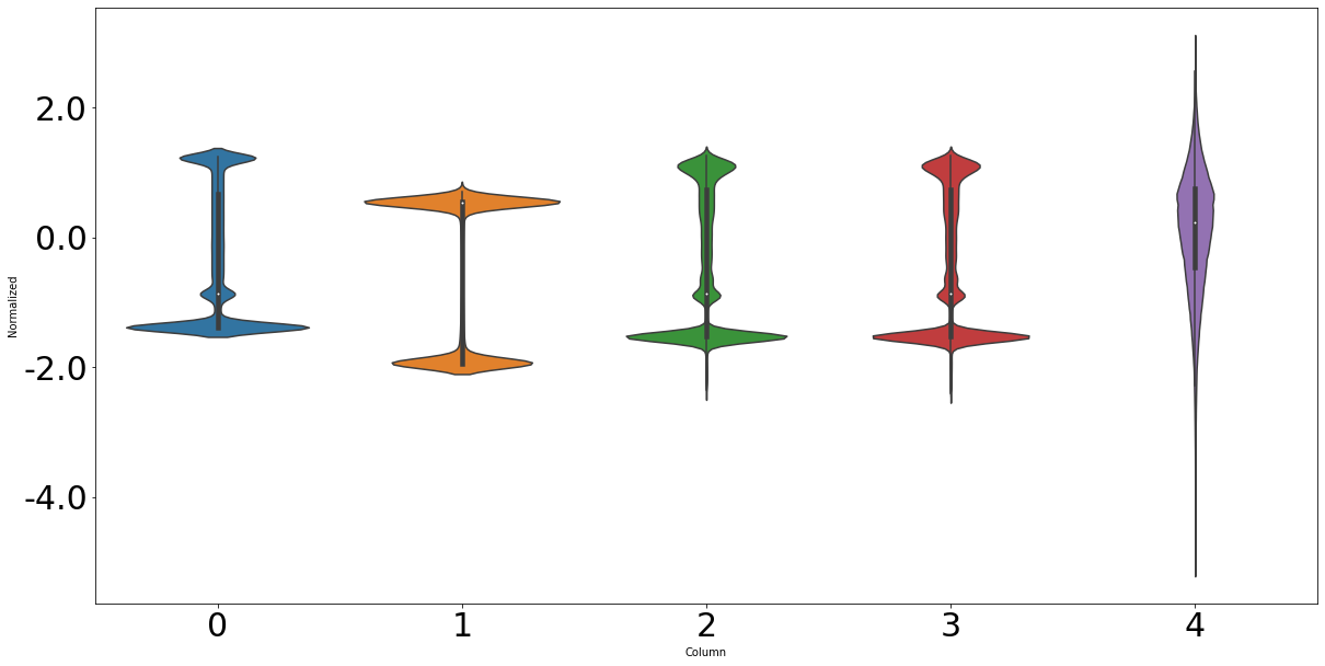
df_std = (df_train - train_mean) / train_std
df_std = df_std.melt(var_name='Column', value_name='Normalized')

fig, ax = plt.subplots(figsize=[20, 10])
ax = sns.violinplot(x='Column', y='Normalized', data=df_std)
ax.set_xticklabels(ax.get_xticks(), size = 30)
ax.set_yticklabels(ax.get_yticks(), size = 30)

<ipython-input-19-bf96d0c125a6>:31: UserWarning: FixedFormatter should only be used together with FixedLocator
  ax.set_yticklabels(ax.get_yticks(), size = 30)

[Text(0, -6.0, '-6.0'),
 Text(0, -4.0, '-4.0'),
 Text(0, -2.0, '-2.0'),
 Text(0, 0.0, '0.0'),
 Text(0, 2.0, '2.0'),
 Text(0, 4.0, '4.0')]

4, Dataset (rolling/windowed dataset) for time series analysis

4.1, Read data into the data class

# 4.1.1, Indexes and offsets

## NB: the data for training, testing and validation should be store here first!!
class WindowGenerator():
  def __init__(self, input_width, label_width, shift,
               train_df=train_df, val_df=val_df, test_df=test_df,
               label_columns=None):
    # Store the raw data.
    self.train_df = train_df
    self.val_df = val_df
    self.test_df = test_df

    # Work out the label column indices.
    self.label_columns = label_columns
    if label_columns is not None:
      self.label_columns_indices = {name: i for i, name in
                                    enumerate(label_columns)}
    self.column_indices = {name: i for i, name in
                           enumerate(train_df.columns)}

    # Work out the window parameters.
    self.input_width = input_width
    self.label_width = label_width
    self.shift = shift

    self.total_window_size = input_width + shift

    self.input_slice = slice(0, input_width)
    self.input_indices = np.arange(self.total_window_size)[self.input_slice]

    self.label_start = self.total_window_size - self.label_width
    self.labels_slice = slice(self.label_start, None)
    self.label_indices = np.arange(self.total_window_size)[self.labels_slice]

  def __repr__(self):
    return '\n'.join([
        f'Total window size: {self.total_window_size}',
        f'Input indices: {self.input_indices}',
        f'Label indices: {self.label_indices}',
        f'Label column name(s): {self.label_columns}'])

# 4.1.2, Split the window
def split_window(self, features):
  inputs = features[:, self.input_slice, :]
  labels = features[:, self.labels_slice, :]
  if self.label_columns is not None:
    labels = tf.stack(
        [labels[:, :, self.column_indices[name]] for name in self.label_columns],
        axis=-1)

  # Slicing doesn't preserve static shape information, so set the shapes
  # manually. This way the `tf.data.Datasets` are easier to inspect.
  inputs.set_shape([None, self.input_width, None])
  labels.set_shape([None, self.label_width, None])

  return inputs, labels

WindowGenerator.split_window = split_window


# 4.1.3, plot the time series  ################# NB: this also needs to set up the label/output parameter
def plot(self, model=None, plot_col='head_gross', max_subplots=3):
  inputs, labels = self.example
  plt.figure(figsize=(12, 8))
  plot_col_index = self.column_indices[plot_col]
  max_n = min(max_subplots, len(inputs))
  for n in range(max_n):
    plt.subplot(max_n, 1, n+1)
    plt.ylabel(f'{plot_col} [normed]')
    plt.plot(self.input_indices, inputs[n, :, plot_col_index],
             label='Inputs', marker='.', zorder=-10)

    if self.label_columns:
      label_col_index = self.label_columns_indices.get(plot_col, None)
    else:
      label_col_index = plot_col_index

    if label_col_index is None:
      continue

    plt.scatter(self.label_indices, labels[n, :, label_col_index],
                edgecolors='k', label='Labels', c='#2ca02c', s=64)
    if model is not None:
      predictions = model(inputs)
      plt.scatter(self.label_indices, predictions[n, :, label_col_index],
                  marker='X', edgecolors='k', label='Predictions',
                  c='#ff7f0e', s=64)

    if n == 0:
      plt.legend()

  plt.xlabel('Time [minisecond]')

WindowGenerator.plot = plot

4.2, Check the constructed basic dataset class

# Test of windowed dataset 

#w0 = WindowGenerator(input_width=24, label_width=1, shift=24, label_columns=['head_gross'])
w1 = WindowGenerator(input_width=24, label_width=1, shift=24, label_columns=None)
w=w1

# Stack three slices, the length of the total window.
example_window = tf.stack([np.array(train_df[:w.total_window_size]),
                           np.array(train_df[100:100+w.total_window_size]),
                           np.array(train_df[200:200+w.total_window_size])])

example_inputs, example_labels = w.split_window(example_window)

print('All shapes are: (batch, time, features)')
print(f'Window shape: {example_window.shape}')
print(f'Inputs shape: {example_inputs.shape}')
print(f'Labels shape: {example_labels.shape}')

All shapes are: (batch, time, features)
Window shape: (3, 48, 5)
Inputs shape: (3, 24, 5)
Labels shape: (3, 1, 5)

w.example = example_inputs, example_labels
w.plot(plot_col='guide_open')

4.3, Formulate train, test, validation datasets in the data structure

def make_dataset(self, data):
  data = np.array(data, dtype=np.float32)
  ds = tf.keras.preprocessing.timeseries_dataset_from_array(
      data=data,
      targets=None,
      sequence_length=self.total_window_size,
      sequence_stride=1,
      shuffle=True,
      batch_size=32,)

  ds = ds.map(self.split_window)

  return ds

WindowGenerator.make_dataset = make_dataset

# add properties to the dataset
@property
def train(self):
  return self.make_dataset(self.train_df)

@property
def val(self):
  return self.make_dataset(self.val_df)

@property
def test(self):
  return self.make_dataset(self.test_df)

@property
def example(self):
  """Get and cache an example batch of `inputs, labels` for plotting."""
  result = getattr(self, '_example', None)
  if result is None:
    # No example batch was found, so get one from the `.train` dataset
    result = next(iter(self.train))
    # And cache it for next time
    self._example = result
  return result

WindowGenerator.train = train
WindowGenerator.val = val
WindowGenerator.test = test
WindowGenerator.example = example

# Run the example to get the index
for example_inputs, example_labels in w.train.take(1):
  print(f'Inputs shape (batch, time, features): {example_inputs.shape}')
  print(f'Labels shape (batch, time, features): {example_labels.shape}')

Inputs shape (batch, time, features): (32, 24, 5)
Labels shape (batch, time, features): (32, 1, 5)

for example_inputs, example_labels in w.train.take(1):
  print(f'Inputs shape (batch, time, features): {example_inputs.shape}')
  print(f'Labels shape (batch, time, features): {example_labels.shape}')

Inputs shape (batch, time, features): (32, 24, 5)
Labels shape (batch, time, features): (32, 1, 5)

5, Single step model: $\(Head\_t = f(guide\_open_{(t-1, t-2, ...)}, pump\_speed_{(t-1, t-2, ...)}, discharge\_rate_{(t-1, t-2, ...)},...)\)$

5.1, Baseline and linear models

Baseline narrow window	Baseline wide window	Linear model with narrow window	Linear model with wide window

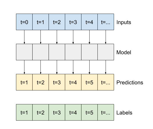
Test 1: narrow window dataset (single output window)

# Get the first dataset (all features as output)
single_step_window = WindowGenerator(
    input_width=1, label_width=1, shift=1,
    label_columns = ['head_gross']) # we can set "label_columns=None"
single_step_window

for example_inputs, example_labels in single_step_window.train.take(1):
  print(f'Inputs shape (batch, time, features): {example_inputs.shape}')
  print(f'Labels shape (batch, time, features): {example_labels.shape}')
    
single_step_window.label_columns, single_step_window.column_indices

Inputs shape (batch, time, features): (32, 1, 5)
Labels shape (batch, time, features): (32, 1, 1)

(['head_gross'],
 {'guide_open': 0,
  'running_speed': 1,
  'pump101_speed': 2,
  'pump102_speed': 3,
  'head_gross': 4})

# Baseline model
class Baseline(tf.keras.Model):
  def __init__(self, label_index=None):
    super().__init__()
    self.label_index = label_index

  def call(self, inputs):
    if self.label_index is None:
      return inputs
    result = inputs[:, :, self.label_index]
    return result[:, :, tf.newaxis]

# Build the model
baseline = Baseline(label_index=single_step_window.column_indices['head_gross'])

#baseline = Baseline(label_index=None)

baseline.compile(loss=tf.losses.MeanSquaredError(),
                 metrics=[tf.metrics.MeanAbsoluteError()])

val_performance = {}
performance = {}
val_performance['Baseline'] = baseline.evaluate(single_step_window.val)
performance['Baseline'] = baseline.evaluate(single_step_window.test, verbose=0)

2458/2458 [==============================] - 4s 2ms/step - loss: 0.0034 - mean_absolute_error: 0.0432

single_step_window.test

<MapDataset shapes: ((None, 1, 5), (None, 1, 1)), types: (tf.float32, tf.float32)>

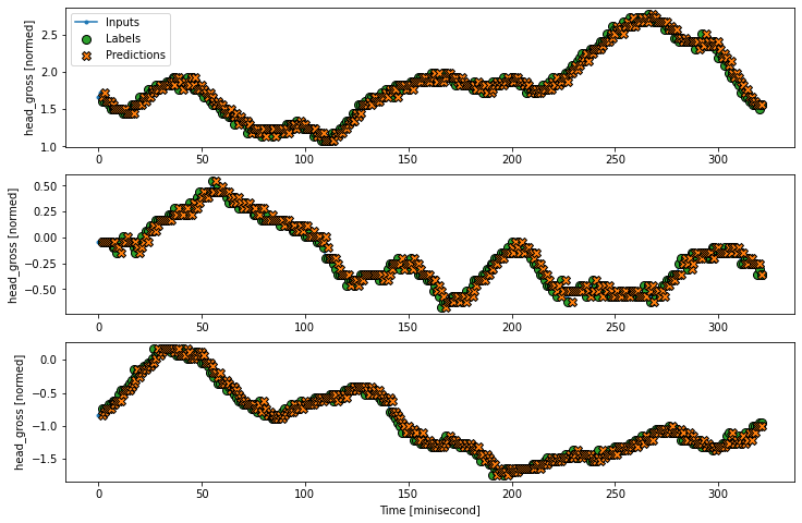
Test 2: wide output window

wide_window = WindowGenerator(
    input_width=320, label_width=320, shift=2,
    label_columns=['head_gross'])    ################# NB: it is very important to choose the parameters here ##############
###################################################################################################################################

wide_window.plot(baseline)

From above analysis, it should be remarked

• it is important to keep “baseline = Baseline(label_index=single_step_window.column_indices[‘head_gross’])”

• the index should be the same as the WindowGenerator function!!***

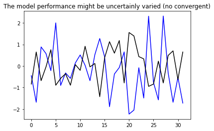
5.2, Linear model with narrow window dataset ”WindowGenerator(input_width=1, label_width=1, shift=1)”

# define linear model from the package
linear = tf.keras.Sequential([
    tf.keras.layers.Dense(units=1)
])

# Check the linear model
print('Input shape:', single_step_window.example[0].shape)
print('Output shape:', linear(single_step_window.example[0]).shape)

# Plot the result to check the linear model
plt.plot(linear(single_step_window.example[0]).numpy().flatten(), 'b') 
plt.plot(single_step_window.example[1].numpy().flatten(), 'k')
plt.title('The model performance might be uncertainly varied (no convergent)')
plt.show()

Input shape: (32, 1, 5)
Output shape: (32, 1, 1)

MAX_EPOCHS = 3

def compile_and_fit(model, window, patience=2):
  early_stopping = tf.keras.callbacks.EarlyStopping(monitor='val_loss',
                                                    patience=patience,
                                                    mode='min')

  model.compile(loss=tf.losses.MeanSquaredError(),
                optimizer=tf.optimizers.Adam(),
                metrics=[tf.metrics.MeanAbsoluteError()])

  history = model.fit(window.train, epochs=MAX_EPOCHS,
                      validation_data=window.val,
                      callbacks=[early_stopping])
  return history

history = compile_and_fit(linear, single_step_window)

val_performance['Linear'] = linear.evaluate(single_step_window.val)
performance['Linear'] = linear.evaluate(single_step_window.test, verbose=0)

Epoch 1/3
17204/17204 [==============================] - 54s 3ms/step - loss: 0.1395 - mean_absolute_error: 0.1352 - val_loss: 0.0035 - val_mean_absolute_error: 0.0460
Epoch 2/3
17204/17204 [==============================] - 52s 3ms/step - loss: 0.0037 - mean_absolute_error: 0.0467 - val_loss: 0.0034 - val_mean_absolute_error: 0.0449
Epoch 3/3
17204/17204 [==============================] - 52s 3ms/step - loss: 0.0036 - mean_absolute_error: 0.0463 - val_loss: 0.0036 - val_mean_absolute_error: 0.0486
2458/2458 [==============================] - 5s 2ms/step - loss: 0.0036 - mean_absolute_error: 0.0486

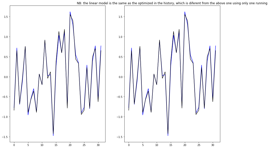
# Two ways to plot the results

fig, (ax1, ax2) = plt.subplots(1,2, figsize = [15, 10])
# first plot based on the iteractive model
ax1.plot(history.model.predict(single_step_window.example[0]).flatten(),'b')
ax1.plot(single_step_window.example[1].numpy().flatten(), 'k')

# second plot based on the 
ax2.plot(linear(single_step_window.example[0]).numpy().flatten(), 'b') 
ax2.plot(single_step_window.example[1].numpy().flatten(), 'k')
ax2.set_title("NB: the linear model is the same as the optimized in the history, which is diferent from the above one using only one running")

Text(0.5, 1.0, 'NB: the linear model is the same as the optimized in the history, which is diferent from the above one using only one running')

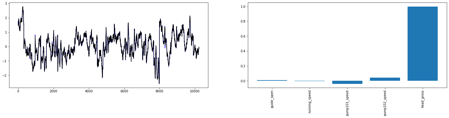
5.3, linear model for wide window data inputs ”WindowGenerator(input_width=300, label_width=300, shift=1)”

# Plot the result to check the linear model
fig, (ax1, ax2) = plt.subplots(1,2,figsize=(25,5))
ax1.plot(linear(wide_window.example[0]).numpy().flatten(), 'b') 
ax1.plot(wide_window.example[1].numpy().flatten(), 'k')


# plot the weight bars used in this model
ax2.bar(x = range(len(train_df.columns)),
        height=linear.layers[0].kernel[:,0].numpy())
#axis = plt.gca()
ax2.set_xticks(range(len(train_df.columns)))
_ = ax2.set_xticklabels(train_df.columns, rotation=90)
#plt.show()

# Lets make the wider window dataset
wide_window.plot(linear)
print('Input shape:', wide_window.example[0].shape)
print('Output shape:', baseline(wide_window.example[0]).shape)

Input shape: (32, 320, 5)
Output shape: (32, 320, 1)

5.4, Dense model (multiple layers and activation function)

Multi-step dense dataset structure

# model construction and estimation
dense = tf.keras.Sequential([
    tf.keras.layers.Dense(units=64, activation='relu'),
    tf.keras.layers.Dense(units=64, activation='relu'),
    tf.keras.layers.Dense(units=1)
])

history = compile_and_fit(dense, single_step_window)

val_performance['Dense'] = dense.evaluate(single_step_window.val)
performance['Dense'] = dense.evaluate(single_step_window.test, verbose=0)

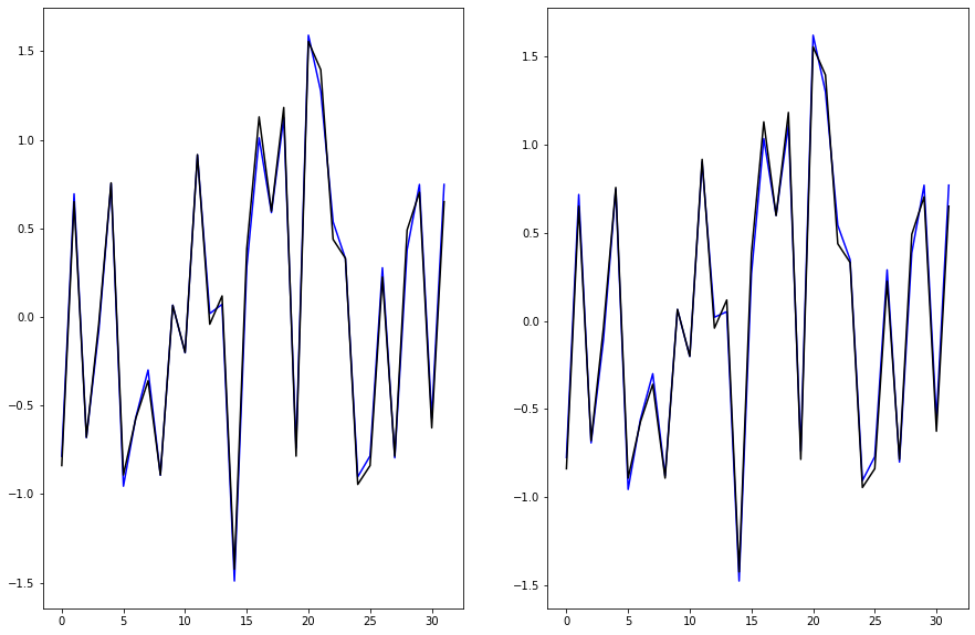
# plot the results
fig, (ax1, ax2) = plt.subplots(1,2, figsize = [15, 10])
# first plot based on the iteractive model
ax1.plot(history.model.predict(single_step_window.example[0]).flatten(),'b')
ax1.plot(single_step_window.example[1].numpy().flatten(), 'k')

# second plot based on the 
ax2.plot(linear(single_step_window.example[0]).numpy().flatten(), 'b') 
ax2.plot(single_step_window.example[1].numpy().flatten(), 'k')

Epoch 1/3
17204/17204 [==============================] - 79s 5ms/step - loss: 0.0047 - mean_absolute_error: 0.0508 - val_loss: 0.0042 - val_mean_absolute_error: 0.0525
Epoch 2/3
17204/17204 [==============================] - 78s 5ms/step - loss: 0.0038 - mean_absolute_error: 0.0486 - val_loss: 0.0035 - val_mean_absolute_error: 0.0462
Epoch 3/3
17204/17204 [==============================] - 78s 5ms/step - loss: 0.0038 - mean_absolute_error: 0.0482 - val_loss: 0.0034 - val_mean_absolute_error: 0.0447
2458/2458 [==============================] - 8s 3ms/step - loss: 0.0034 - mean_absolute_error: 0.0447

[<matplotlib.lines.Line2D at 0x2825537bf40>]

6, CNN Model construction for \(x_t = f(X_{t-1}, X_{t-2}, X_{t-3},...)\)

6.1, Set up the convolutional neuron network (CNN) dataset.

# Create the indexes
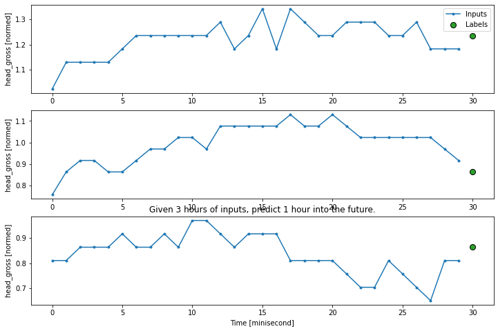
CONV_WIDTH = 30
conv_window = WindowGenerator(
    input_width=CONV_WIDTH,
    label_width=1,
    shift=1,
    label_columns=['head_gross'])

print(conv_window)

# plot the input data/features
conv_window.plot()
plt.title("Given 3 hours of inputs, predict 1 hour into the future.")

Total window size: 31
Input indices: [ 0  1  2  3  4  5  6  7  8  9 10 11 12 13 14 15 16 17 18 19 20 21 22 23
 24 25 26 27 28 29]
Label indices: [30]
Label column name(s): ['head_gross']

Text(0.5, 1.0, 'Given 3 hours of inputs, predict 1 hour into the future.')

6.2, Test for the “multiple-steps model” model

(Using CNN data structure) – Narrow window: input_width = 3

# configure the model
multi_step_dense = tf.keras.Sequential([
    # Shape: (time, features) => (time*features)
    tf.keras.layers.Flatten(),
    tf.keras.layers.Dense(units=32, activation='relu'),
    tf.keras.layers.Dense(units=32, activation='relu'),
    tf.keras.layers.Dense(units=1),
    # Add back the time dimension.
    # Shape: (outputs) => (1, outputs)
    tf.keras.layers.Reshape([1, -1]),
])

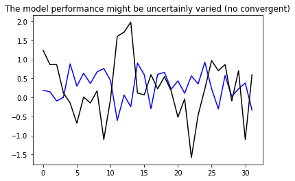
# Plot the result to check the linear model
plt.plot(multi_step_dense(conv_window.example[0]).numpy().flatten(), 'b') 
plt.plot(conv_window.example[1].numpy().flatten(), 'k')
plt.title('The model performance might be uncertainly varied (no convergent)')
plt.show()

# optimise the model through "compile_and_fit"
import IPython

history = compile_and_fit(multi_step_dense, conv_window)

IPython.display.clear_output()
val_performance['Multi step dense'] = multi_step_dense.evaluate(conv_window.val)
performance['Multi step dense'] = multi_step_dense.evaluate(conv_window.test, verbose=0)

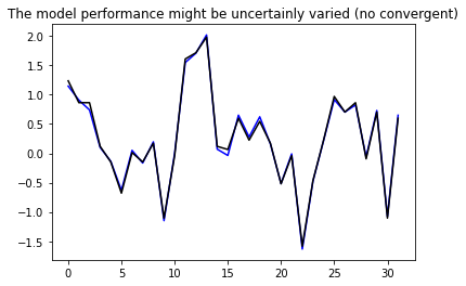
# Plot the result to check the linear model
plt.plot(history.model.predict(conv_window.example[0]).flatten(), 'b') 
plt.plot(conv_window.example[1].numpy().flatten(), 'k')
plt.title('The model performance might be uncertainly varied (no convergent)')
plt.show()

2457/2457 [==============================] - 5s 2ms/step - loss: 0.0028 - mean_absolute_error: 0.0424

6.3, Convolutional Neuron Network:

Narrow window: input_width = CONV_width = 3 Difference between multi-step dense model and CNN model

• model construction: CNN model require input_width, but no need for layers.flatten() and layers.reshape([1, -1])

• data structure: output of CNN datastructure is (#input_window -1) dimensions less

# Configure the CNN model
conv_model = tf.keras.Sequential([
    tf.keras.layers.Conv1D(filters=32,
                           kernel_size=(CONV_WIDTH,),
                           activation='relu'),
    tf.keras.layers.Dense(units=32, activation='relu'),
    tf.keras.layers.Dense(units=1),
])

print("Conv model on `conv_window`")
print('Input shape:', conv_window.example[0].shape)
print('Output shape:', conv_model(conv_window.example[0]).shape)

# Estimate the CNN model
history = compile_and_fit(conv_model, conv_window)

IPython.display.clear_output()
val_performance['Conv'] = conv_model.evaluate(conv_window.val)
performance['Conv'] = conv_model.evaluate(conv_window.test, verbose=0)

2457/2457 [==============================] - 8s 3ms/step - loss: 0.0031 - mean_absolute_error: 0.0449

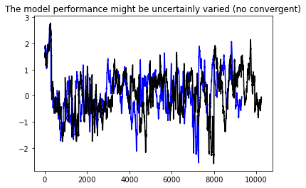
# Check the length difference between multiple-step-dense model and the CNN model
print("Wide window")
print('Input shape:', wide_window.example[0].shape)
print('Labels shape:', wide_window.example[1].shape)
print('Output shape:', conv_model(wide_window.example[0]).shape)

#  Plot the result to check the linear model
plt.plot(history.model.predict(wide_window.example[0]).flatten(), 'b') 
plt.plot(wide_window.example[1].numpy().flatten(), 'k')
plt.title('The model performance might be uncertainly varied (no convergent)')
plt.show()

Wide window
Input shape: (32, 320, 5)
Labels shape: (32, 320, 1)
Output shape: (32, 291, 1)
WARNING:tensorflow:5 out of the last 66 calls to <function Model.make_predict_function.<locals>.predict_function at 0x0000028256AB3A60> triggered tf.function retracing. Tracing is expensive and the excessive number of tracings could be due to (1) creating @tf.function repeatedly in a loop, (2) passing tensors with different shapes, (3) passing Python objects instead of tensors. For (1), please define your @tf.function outside of the loop. For (2), @tf.function has experimental_relax_shapes=True option that relaxes argument shapes that can avoid unnecessary retracing. For (3), please refer to https://www.tensorflow.org/guide/function#controlling_retracing and https://www.tensorflow.org/api_docs/python/tf/function for  more details.

6.4, Convolutional Neuron Network

Wide window: input_width = CONV_width = 30

LABEL_WIDTH = 24
INPUT_WIDTH = LABEL_WIDTH + (CONV_WIDTH - 1)
wide_conv_window = WindowGenerator(
    input_width=INPUT_WIDTH,
    label_width=LABEL_WIDTH,
    shift=1,
    label_columns=['head_gross'])

wide_conv_window
print("Wide conv window")
print('Input shape:', wide_conv_window.example[0].shape)
print('Labels shape:', wide_conv_window.example[1].shape)
print('Output shape:', conv_model(wide_conv_window.example[0]).shape)
wide_conv_window.plot(conv_model)

Wide conv window
Input shape: (32, 53, 5)
Labels shape: (32, 24, 1)
Output shape: (32, 24, 1)

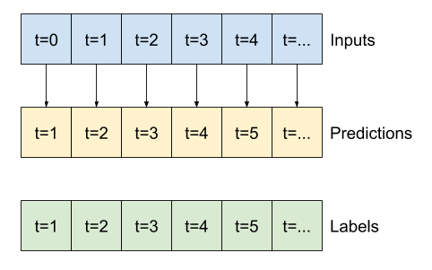
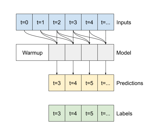
6.5 Recurrent Neuron Network (RNN)

In this example test, we will use the LSTM of RNN for demonstration

Input: Data structure of the RNN input	Output: only the final results	Output: all internal prediction results

Difference between second output and third outpus

• return_sequences=False for the second figure above

• return_sequences=True for the third figure above

# Configure the RNN (LSTM) model
lstm_model = tf.keras.models.Sequential([
    # Shape [batch, time, features] => [batch, time, lstm_units]
    tf.keras.layers.LSTM(32, return_sequences=False),
    # Shape => [batch, time, features]
    tf.keras.layers.Dense(units=1)
])

print('Input shape:', wide_window.example[0].shape)
print('Output shape:', lstm_model(wide_window.example[0]).shape)

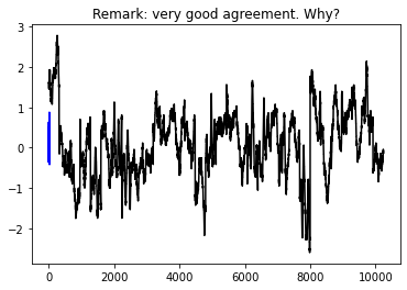
#  Plot the result to check the linear model
plt.plot(lstm_model(wide_window.example[0]).numpy().flatten(), 'b') 
plt.plot(wide_window.example[1].numpy().flatten(), 'k')
plt.title('Remark: very good agreement. Why?')
plt.show()

Input shape: (32, 320, 5)
Output shape: (32, 1)

'''
# Estimate/construct the model
history_lstm = compile_and_fit(lstm_model, wide_window)

IPython.display.clear_output()
val_performance['LSTM'] = lstm_model.evaluate(wide_window.val)
performance['LSTM'] = lstm_model.evaluate(wide_window.test, verbose=0)

### It seems that the RNN cannot be run at CPU computers
### Tests from other websites
##batch_size = 100
##from tensorflow.keras import Sequential
##from tensorflow.keras.layers import LSTM, Dense
##from tensorflow.keras.optimizers import Adam
##
##model = Sequential()
##model.add(LSTM(100, batch_input_shape=(32, 320, 5), return_sequences=True))
##model.add(LSTM(100, return_sequences=True))
##model.add(LSTM(100))
##model.add(Dense(number_of_classes, activation='softmax'))
##
##model.summary()
##
##print("Created model.")
##
##model.compile(optimizer=Adam(lr=0.02),
##              loss='categorical_crossentropy', 
##              metrics=['acc'])
##
##print("Compiled model.")

'''

'\n# Estimate/construct the model\nhistory_lstm = compile_and_fit(lstm_model, wide_window)\n\nIPython.display.clear_output()\nval_performance[\'LSTM\'] = lstm_model.evaluate(wide_window.val)\nperformance[\'LSTM\'] = lstm_model.evaluate(wide_window.test, verbose=0)\n\n### It seems that the RNN cannot be run at CPU computers\n### Tests from other websites\n##batch_size = 100\n##from tensorflow.keras import Sequential\n##from tensorflow.keras.layers import LSTM, Dense\n##from tensorflow.keras.optimizers import Adam\n##\n##model = Sequential()\n##model.add(LSTM(100, batch_input_shape=(32, 320, 5), return_sequences=True))\n##model.add(LSTM(100, return_sequences=True))\n##model.add(LSTM(100))\n##model.add(Dense(number_of_classes, activation=\'softmax\'))\n##\n##model.summary()\n##\n##print("Created model.")\n##\n##model.compile(optimizer=Adam(lr=0.02),\n##              loss=\'categorical_crossentropy\', \n##              metrics=[\'acc\'])\n##\n##print("Compiled model.")\n\n'

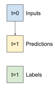
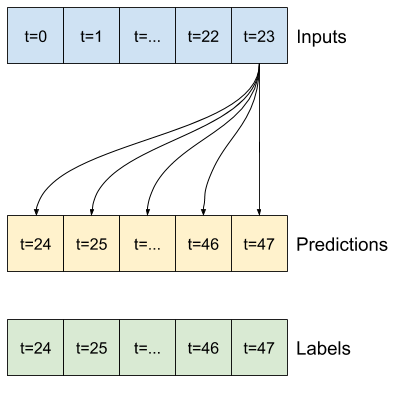
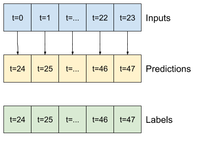
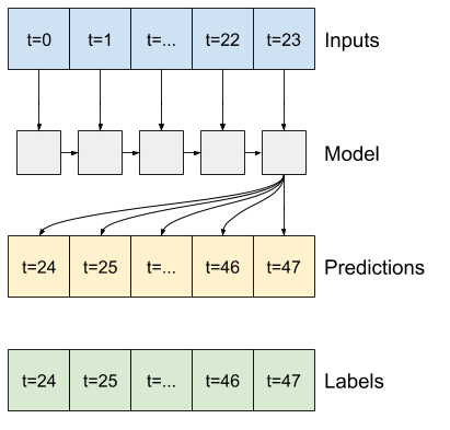
7. Multi-step output models

NB: different from Multi-output models that can be obtained by the previous code. Two rough approaches to this:

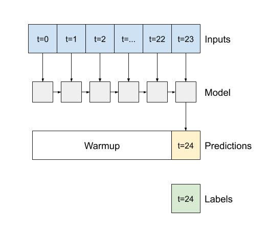
• Single shot predictions where the entire time series is predicted at once.

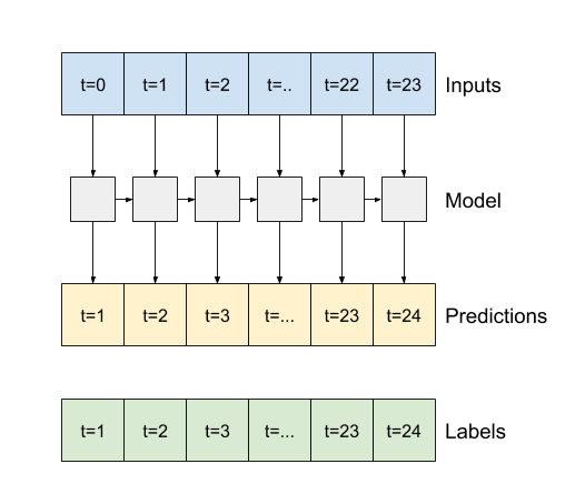
• Autoregressive predictions where the model only makes single step predictions and its output is fed back as its input.

7.1, Generate the dataset for the modelling

NB: we will skip the baseline model in this example

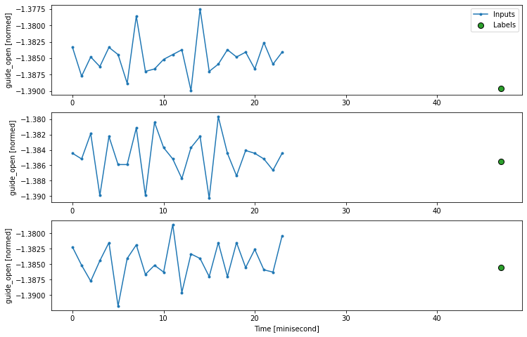
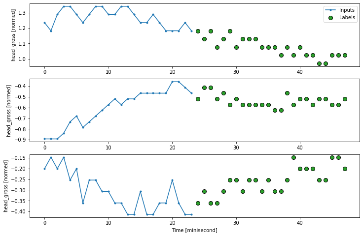
OUT_STEPS = 24
multi_window = WindowGenerator(input_width=24,
                               label_width=OUT_STEPS,
                               shift=OUT_STEPS)

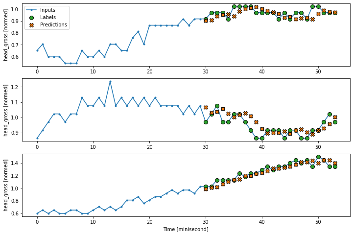
multi_window.plot()
multi_window

Total window size: 48
Input indices: [ 0  1  2  3  4  5  6  7  8  9 10 11 12 13 14 15 16 17 18 19 20 21 22 23]
Label indices: [24 25 26 27 28 29 30 31 32 33 34 35 36 37 38 39 40 41 42 43 44 45 46 47]
Label column name(s): None

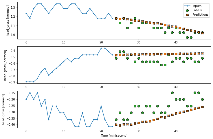
7.2 Illustration of various models for single-shot prediction

base_future = last	base_future = repeated	linear/dense models	CNN	RNN

7.2.1, Linear and dense model

## Linear model
#num_features = df_train.shape[1]
#multi_linear_model = tf.keras.Sequential([
#    # Take the last time-step.
#    # Shape [batch, time, features] => [batch, 1, features]
#    tf.keras.layers.Lambda(lambda x: x[:, -1:, :]),
#    # Shape => [batch, 1, out_steps*features]
#    tf.keras.layers.Dense(OUT_STEPS*num_features,
#                          kernel_initializer=tf.initializers.zeros()),
#    # Shape => [batch, out_steps, features]
#    tf.keras.layers.Reshape([OUT_STEPS, num_features])
#])
#
#history = compile_and_fit(multi_linear_model, multi_window)

multi_val_performance = {}
multi_performance = {}

IPython.display.clear_output()
multi_val_performance['Linear'] = multi_linear_model.evaluate(multi_window.val)
multi_performance['Linear'] = multi_linear_model.evaluate(multi_window.test, verbose=0)
multi_window.plot(multi_linear_model)



# Dense model
multi_dense_model = tf.keras.Sequential([
    # Take the last time step.
    # Shape [batch, time, features] => [batch, 1, features]
    tf.keras.layers.Lambda(lambda x: x[:, -1:, :]),
    # Shape => [batch, 1, dense_units]
    tf.keras.layers.Dense(512, activation='relu'),
    # Shape => [batch, out_steps*features]
    tf.keras.layers.Dense(OUT_STEPS*num_features,
                          kernel_initializer=tf.initializers.zeros()),
    # Shape => [batch, out_steps, features]
    tf.keras.layers.Reshape([OUT_STEPS, num_features])
])

history = compile_and_fit(multi_dense_model, multi_window)

IPython.display.clear_output()
multi_val_performance['Dense'] = multi_dense_model.evaluate(multi_window.val)
multi_performance['Dense'] = multi_dense_model.evaluate(multi_window.test, verbose=0)
multi_window.plot(multi_dense_model)

2457/2457 [==============================] - 7s 3ms/step - loss: 0.0069 - mean_absolute_error: 0.0350

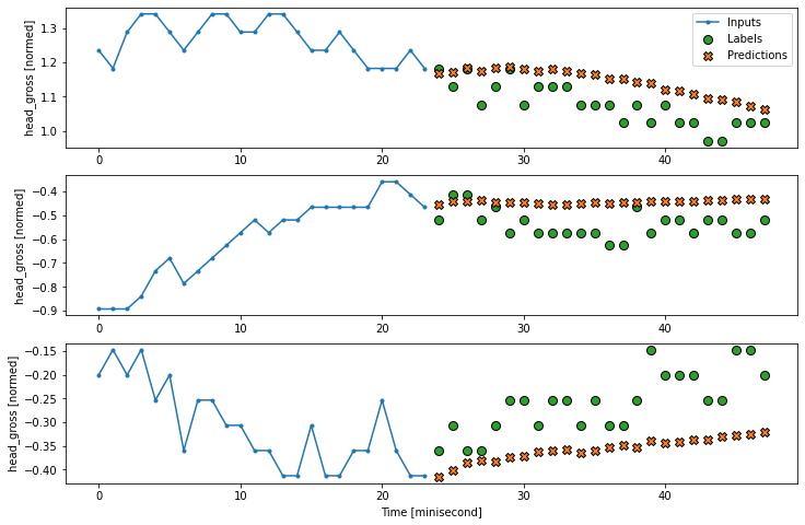
7.2.2, CNN model with conv length

CONV_WIDTH = 3
multi_conv_model = tf.keras.Sequential([
    # Shape [batch, time, features] => [batch, CONV_WIDTH, features]
    tf.keras.layers.Lambda(lambda x: x[:, -CONV_WIDTH:, :]),
    # Shape => [batch, 1, conv_units]
    tf.keras.layers.Conv1D(256, activation='relu', kernel_size=(CONV_WIDTH)),
    # Shape => [batch, 1,  out_steps*features]
    tf.keras.layers.Dense(OUT_STEPS*num_features,
                          kernel_initializer=tf.initializers.zeros()),
    # Shape => [batch, out_steps, features]
    tf.keras.layers.Reshape([OUT_STEPS, num_features])
])

history = compile_and_fit(multi_conv_model, multi_window)

IPython.display.clear_output()

multi_val_performance['Conv'] = multi_conv_model.evaluate(multi_window.val)
multi_performance['Conv'] = multi_conv_model.evaluate(multi_window.test, verbose=0)
multi_window.plot(multi_conv_model)

2457/2457 [==============================] - 6s 3ms/step - loss: 0.0066 - mean_absolute_error: 0.0335

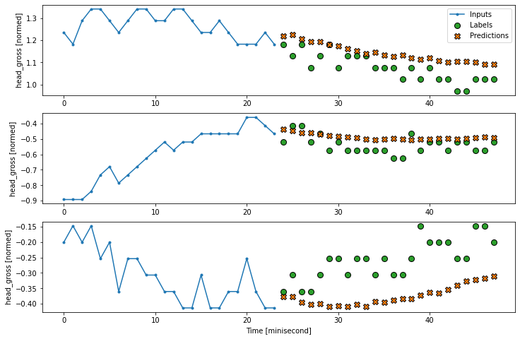
7.3.3, RNN (LSTM) model

multi_lstm_model = tf.keras.Sequential([
    # Shape [batch, time, features] => [batch, lstm_units].
    # Adding more `lstm_units` just overfits more quickly.
    tf.keras.layers.LSTM(32, return_sequences=False),
    # Shape => [batch, out_steps*features].
    tf.keras.layers.Dense(OUT_STEPS*num_features,
                          kernel_initializer=tf.initializers.zeros()),
    # Shape => [batch, out_steps, features].
    tf.keras.layers.Reshape([OUT_STEPS, num_features])
])

history = compile_and_fit(multi_lstm_model, multi_window)

IPython.display.clear_output()

multi_val_performance['LSTM'] = multi_lstm_model.evaluate(multi_window.val)
multi_performance['LSTM'] = multi_lstm_model.evaluate(multi_window.test, verbose=0)
multi_window.plot(multi_lstm_model)

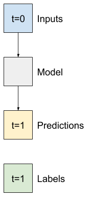
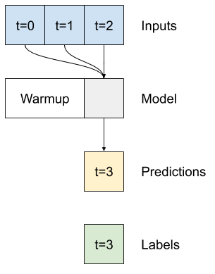
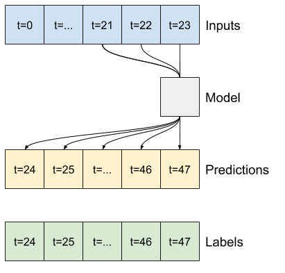
7.3 Illustration of autoregressive RNN model

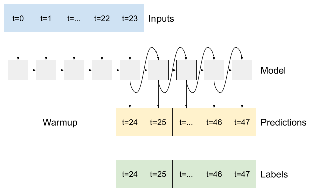
Model description of autoregressive rnn model

# define the model
class FeedBack(tf.keras.Model):
  def __init__(self, units, out_steps):
    super().__init__()
    self.out_steps = out_steps
    self.units = units
    self.lstm_cell = tf.keras.layers.LSTMCell(units)
    # Also wrap the LSTMCell in an RNN to simplify the `warmup` method.
    self.lstm_rnn = tf.keras.layers.RNN(self.lstm_cell, return_state=True)
    self.dense = tf.keras.layers.Dense(num_features)
    
feedback_model = FeedBack(units=32, out_steps=OUT_STEPS)

# define the warm-up
def warmup(self, inputs):
  # inputs.shape => (batch, time, features)
  # x.shape => (batch, lstm_units)
  x, *state = self.lstm_rnn(inputs)

  # predictions.shape => (batch, features)
  prediction = self.dense(x)
  return prediction, state

FeedBack.warmup = warmup
prediction, state = feedback_model.warmup(multi_window.example[0])
prediction.shape


# get iteractive output
def call(self, inputs, training=None):
  # Use a TensorArray to capture dynamically unrolled outputs.
  predictions = []
  # Initialize the LSTM state.
  prediction, state = self.warmup(inputs)

  # Insert the first prediction.
  predictions.append(prediction)

  # Run the rest of the prediction steps.
  for n in range(1, self.out_steps):
    # Use the last prediction as input.
    x = prediction
    # Execute one lstm step.
    x, state = self.lstm_cell(x, states=state,
                              training=training)
    # Convert the lstm output to a prediction.
    prediction = self.dense(x)
    # Add the prediction to the output.
    predictions.append(prediction)

  # predictions.shape => (time, batch, features)
  predictions = tf.stack(predictions)
  # predictions.shape => (batch, time, features)
  predictions = tf.transpose(predictions, [1, 0, 2])
  return predictions

FeedBack.call = call

print('Output shape (batch, time, features): ', feedback_model(multi_window.example[0]).shape)


# train the model
history = compile_and_fit(feedback_model, multi_window)

IPython.display.clear_output()

multi_val_performance['AR LSTM'] = feedback_model.evaluate(multi_window.val)
multi_performance['AR LSTM'] = feedback_model.evaluate(multi_window.test, verbose=0)
multi_window.plot(feedback_model)