Lecture 2 Excercise – 2D regression exercise after the class

• 1, you can use the mathematical formulas to estimate the regression coefficients

• 2, you can also use the sklearn machine learning library for the regression

• In the exercise, we provide the solution for the first option, Your task is to use the SKLEARN library to solve the regression and write a short summary

from __future__ import print_function, division
from builtins import range
# Note: you may need to update your version of future
# sudo pip install -U future


import numpy as np
from mpl_toolkits.mplot3d import Axes3D
import matplotlib.pyplot as plt

# load the data
X = []
Y = []
for line in open('data_2d.csv'):
    x1, x2, y = line.split(',')
    X.append([float(x1), float(x2), 1]) # add the bias term
    Y.append(float(y))

# let's turn X and Y into numpy arrays since that will be useful later
X = np.array(X)
Y = np.array(Y)


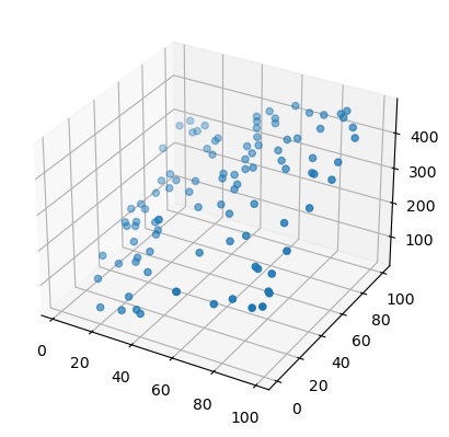
# let's plot the data to see what it looks like
fig = plt.figure()
ax = fig.add_subplot(111, projection='3d')
ax.scatter(X[:,0], X[:,1], Y)
plt.show()

X.shape, Y.shape

((100, 3), (100,))

# apply the equations we learned to calculate a and b
# numpy has a special method for solving Ax = b
# so we don't use x = inv(A)*b
# note: the * operator does element-by-element multiplication in numpy
#       np.dot() does what we expect for matrix multiplication
w = np.linalg.solve(np.dot(X.T, X), np.dot(X.T, Y))
Yhat = np.dot(X, w)


# determine how good the model is by computing the r-squared
d1 = Y - Yhat
d2 = Y - Y.mean()
r2 = 1 - d1.dot(d1) / d2.dot(d2)
print("the r-squared is:", r2)

the r-squared is: 0.9980040612475777