Lecture 5: Examples of GLM and GAM#
GLM: Generalized Linear Models (logical regression is a special GLM)
GAM: Generalized Additive Models
Part I: GLM#
Generalized linear models of different kinds are used based on the probability distribution of the response variables:
GLM is particularly useful when the response variable is not normally distributed or when the relationship between the predictor variables and the response variable is non-linear.
import matplotlib.pyplot as plt
import numpy as np
from sklearn.linear_model import LinearRegression
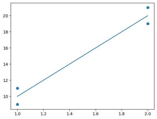
x = [[1], [1], [2], [2]]
y = [9, 11, 19, 21]
m = LinearRegression()
m.fit(x, y)
m.predict([[1]]) # Returns 10
m.predict([[2]]) # Returns 20
m.intercept_, m.coef_
plt.scatter(x,y)
plt.plot(x,m.predict(x))
plt.show()

from sklearn.linear_model import LinearRegression
x = [[7],[8],[9]]
y = [0.50, 0.40, 0.30]
m = LinearRegression()
m.fit(x, y)
m.predict([[1], [20]]) # Returns 110% and -80%
array([ 1.1, -0.8])
If the model give unrealistic extrapolation results, transformations of the model’s inputs or outputs could help to add the constraints, such as put the data into a logarithmic scale and hope for your model to work.
A link function, that links E(y|x) to the linear equation.
The targets follow an exponential distribution. The normal distribution is just one member of this exponential family.
Poission Regression and Gamma Regression are two good examples
1.1, Poission regression#
The French Motor Third-Party Liability Claims dataset#
This is the example from Scikit learn website (https://scikit-learn.org/stable/auto_examples/linear_model/plot_poisson_regression_non_normal_loss.html#sphx-glr-auto-examples-linear-model-plot-poisson-regression-non-normal-loss-py) provided by
Authors:
import numpy as np
import matplotlib.pyplot as plt
import pandas as pd
from sklearn.datasets import fetch_openml


df = fetch_openml(data_id=41214, as_frame=True, parser="pandas").frame
df
| IDpol | ClaimNb | Exposure | Area | VehPower | VehAge | DrivAge | BonusMalus | VehBrand | VehGas | Density | Region | |
|---|---|---|---|---|---|---|---|---|---|---|---|---|
| 0 | 1.0 | 1 | 0.10000 | D | 5 | 0 | 55 | 50 | B12 | 'Regular' | 1217 | R82 |
| 1 | 3.0 | 1 | 0.77000 | D | 5 | 0 | 55 | 50 | B12 | 'Regular' | 1217 | R82 |
| 2 | 5.0 | 1 | 0.75000 | B | 6 | 2 | 52 | 50 | B12 | 'Diesel' | 54 | R22 |
| 3 | 10.0 | 1 | 0.09000 | B | 7 | 0 | 46 | 50 | B12 | 'Diesel' | 76 | R72 |
| 4 | 11.0 | 1 | 0.84000 | B | 7 | 0 | 46 | 50 | B12 | 'Diesel' | 76 | R72 |
| ... | ... | ... | ... | ... | ... | ... | ... | ... | ... | ... | ... | ... |
| 678008 | 6114326.0 | 0 | 0.00274 | E | 4 | 0 | 54 | 50 | B12 | 'Regular' | 3317 | R93 |
| 678009 | 6114327.0 | 0 | 0.00274 | E | 4 | 0 | 41 | 95 | B12 | 'Regular' | 9850 | R11 |
| 678010 | 6114328.0 | 0 | 0.00274 | D | 6 | 2 | 45 | 50 | B12 | 'Diesel' | 1323 | R82 |
| 678011 | 6114329.0 | 0 | 0.00274 | B | 4 | 0 | 60 | 50 | B12 | 'Regular' | 95 | R26 |
| 678012 | 6114330.0 | 0 | 0.00274 | B | 7 | 6 | 29 | 54 | B12 | 'Diesel' | 65 | R72 |
678013 rows × 12 columns
df["Frequency"] = df["ClaimNb"] / df["Exposure"]

print("Average Frequency = {}".format(np.average(df["Frequency"], weights=df["Exposure"])))

print("Fraction of exposure with zero claims = {0:.1%}".format(df.loc[df["ClaimNb"] == 0, "Exposure"].sum() / df["Exposure"].sum()))

fig, (ax0, ax1, ax2) = plt.subplots(ncols=3, figsize=(16, 4))
ax0.set_title("Number of claims")
_ = df["ClaimNb"].hist(bins=30, log=True, ax=ax0)
ax1.set_title("Exposure in years")
_ = df["Exposure"].hist(bins=30, log=True, ax=ax1)
ax2.set_title("Frequency (number of claims per year)")
_ = df["Frequency"].hist(bins=30, log=True, ax=ax2)
plt.show()
print("Hard to explain and predict the number of claims according to the frequency")
Average Frequency = 0.10070308464041304
Fraction of exposure with zero claims = 93.9%

Hard to explain and predict the number of claims according to the frequency
NB: Depends on which LM the data suit, the key is to have a proper transformation
from sklearn.pipeline import make_pipeline
from sklearn.preprocessing import FunctionTransformer, OneHotEncoder
from sklearn.preprocessing import StandardScaler, KBinsDiscretizer
from sklearn.compose import ColumnTransformer


log_scale_transformer = make_pipeline(FunctionTransformer(np.log, validate=False), StandardScaler())

linear_model_preprocessor = ColumnTransformer(
    [   ("passthrough_numeric", "passthrough", ["BonusMalus"]),
        ("binned_numeric", KBinsDiscretizer(n_bins=10, subsample=int(2e5), random_state=0),
                           ["VehAge", "DrivAge"],),
        ("log_scaled_numeric", log_scale_transformer, ["Density"]),
        ("onehot_categorical", OneHotEncoder(),
                              ["VehBrand", "VehPower", "VehGas", "Region", "Area"],  ),  ],

    remainder="drop",
)
from sklearn.dummy import DummyRegressor
from sklearn.pipeline import Pipeline
from sklearn.model_selection import train_test_split

df_train, df_test = train_test_split(df, test_size=0.33, random_state=0)

dummy = Pipeline(
    [
        ("preprocessor", linear_model_preprocessor),
        ("regressor", DummyRegressor(strategy="mean")),
    ]
).fit(df_train, df_train["Frequency"], regressor__sample_weight=df_train["Exposure"])
from sklearn.metrics import mean_squared_error
from sklearn.metrics import mean_absolute_error
from sklearn.metrics import mean_poisson_deviance


def score_estimator(estimator, df_test):
    """Score an estimator on the test set."""
    y_pred = estimator.predict(df_test)

    print(
        "MSE: %.3f"
        % mean_squared_error(
            df_test["Frequency"], y_pred, sample_weight=df_test["Exposure"]
        )
    )
    print(
        "MAE: %.3f"
        % mean_absolute_error(
            df_test["Frequency"], y_pred, sample_weight=df_test["Exposure"]
        )
    )

    # Ignore non-positive predictions, as they are invalid for
    # the Poisson deviance.
    mask = y_pred > 0
    if (~mask).any():
        n_masked, n_samples = (~mask).sum(), mask.shape[0]
        print(
            "WARNING: Estimator yields invalid, non-positive predictions "
            f" for {n_masked} samples out of {n_samples}. These predictions "
            "are ignored when computing the Poisson deviance."
        )

    print(
        "mean Poisson deviance: %.3f"
        % mean_poisson_deviance(
            df_test["Frequency"][mask],
            y_pred[mask],
            sample_weight=df_test["Exposure"][mask],
        )
    )


print("Constant mean frequency evaluation:")
score_estimator(dummy, df_test)
Constant mean frequency evaluation:
MSE: 0.564
MAE: 0.189
mean Poisson deviance: 0.625
Generalized Linear Models
from sklearn.linear_model import Ridge


ridge_glm = Pipeline(
    [
        ("preprocessor", linear_model_preprocessor),
        ("regressor", Ridge(alpha=1e-6)),
    ]
).fit(df_train, df_train["Frequency"], regressor__sample_weight=df_train["Exposure"])

print("Ridge evaluation:")
score_estimator(ridge_glm, df_test)
Ridge evaluation:
MSE: 0.560
MAE: 0.186
WARNING: Estimator yields invalid, non-positive predictions  for 595 samples out of 223745. These predictions are ignored when computing the Poisson deviance.
mean Poisson deviance: 0.597
Directly fit with Poisson regression
from sklearn.linear_model import PoissonRegressor

n_samples = df_train.shape[0]

poisson_glm = Pipeline(
    [
        ("preprocessor", linear_model_preprocessor),
        ("regressor", PoissonRegressor(alpha=1e-12, solver="newton-cholesky")),
    ]
)
poisson_glm.fit(
    df_train, df_train["Frequency"], regressor__sample_weight=df_train["Exposure"]
)

print("PoissonRegressor evaluation:")
score_estimator(poisson_glm, df_test)
PoissonRegressor evaluation:
MSE: 0.560
MAE: 0.186
mean Poisson deviance: 0.594
Part I: GAM#
GAM: Generalized additive models (combining different models –ANN, Deep Learning)
GAM is more developed in R rather than Python
Another extension of GAM is Mixed Effective Models
import numpy as np
import pandas as pd
from pygam import GAM, PoissonGAM, LinearGAM, s, f, te
from pygam.datasets import chicago
import matplotlib.pyplot as plt


X, y = chicago(return_X_y=True)

gam = PoissonGAM(s(0, n_splines=200) + te(3, 1) + s(2)).fit(X, y)

plt.ion()
plt.rcParams['figure.figsize'] = (12, 8)

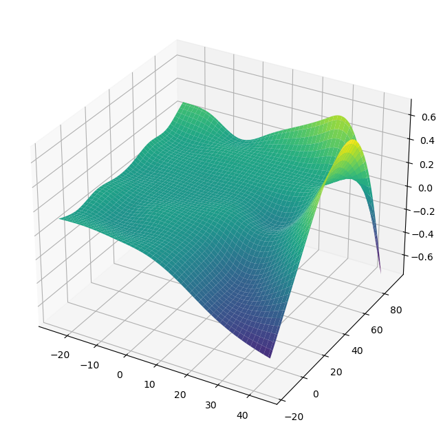
XX = gam.generate_X_grid(term=1, meshgrid=True)
Z = gam.partial_dependence(term=1, X=XX, meshgrid=True)

ax = plt.axes(projection='3d')
ax.plot_surface(XX[0], XX[1], Z, cmap='viridis')
plt.show()

from pygam.datasets import toy_interaction

X, y = toy_interaction(return_X_y=True)

gam = LinearGAM(s(0, by=1)).fit(X, y)
gam.summary()
LinearGAM
=============================================== ==========================================================
Distribution:                        NormalDist Effective DoF:                                     20.8484
Link Function:                     IdentityLink Log Likelihood:                              -2296683.6446
Number of Samples:                        50000 AIC:                                           4593410.986
                                                AICc:                                          4593411.006
                                                GCV:                                                0.0101
                                                Scale:                                              0.0101
                                                Pseudo R-Squared:                                   0.9976
==========================================================================================================
Feature Function                  Lambda               Rank         EDoF         P > x        Sig. Code
================================= ==================== ============ ============ ============ ============
s(0)                              [0.6]                20           19.8         1.11e-16     ***
intercept                                              1            1.0          2.43e-01
==========================================================================================================
Significance codes:  0 '***' 0.001 '**' 0.01 '*' 0.05 '.' 0.1 ' ' 1

WARNING: Fitting splines and a linear function to a feature introduces a model identifiability problem
         which can cause p-values to appear significant when they are not.

WARNING: p-values calculated in this manner behave correctly for un-penalized models or models with
         known smoothing parameters, but when smoothing parameters have been estimated, the p-values
         are typically lower than they should be, meaning that the tests reject the null too readily.
C:\Users\wengang\AppData\Local\Temp\ipykernel_28416\671288597.py:6: UserWarning: KNOWN BUG: p-values computed in this summary are likely much smaller than they should be.

Please do not make inferences based on these values!

Collaborate on a solution, and stay up to date at:
github.com/dswah/pyGAM/issues/163

  gam.summary()
from pygam import LinearGAM, s, f
from pygam.datasets import wage

X, y = wage(return_X_y=True)

## model
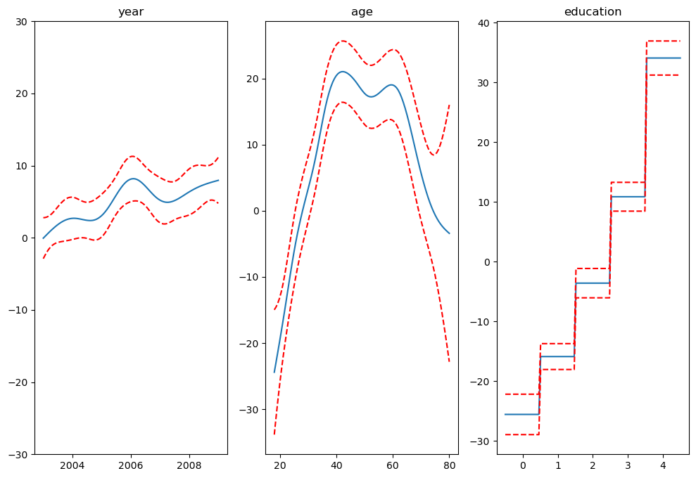
gam = LinearGAM(s(0) + s(1) + f(2))
gam.gridsearch(X, y)


## plotting
plt.figure();
fig, axs = plt.subplots(1,3);

titles = ['year', 'age', 'education']
for i, ax in enumerate(axs):
    XX = gam.generate_X_grid(term=i)
    ax.plot(XX[:, i], gam.partial_dependence(term=i, X=XX))
    ax.plot(XX[:, i], gam.partial_dependence(term=i, X=XX, width=.95)[1], c='r', ls='--')
    if i == 0:
        ax.set_ylim(-30,30)
    ax.set_title(titles[i]);
100% (11 of 11) |########################| Elapsed Time: 0:00:00 Time: 0:00:00
<Figure size 1200x800 with 0 Axes>

gam.summary()
LinearGAM
=============================================== ==========================================================
Distribution:                        NormalDist Effective DoF:                                     19.2602
Link Function:                     IdentityLink Log Likelihood:                                -24116.7451
Number of Samples:                         3000 AIC:                                            48274.0107
                                                AICc:                                           48274.2999
                                                GCV:                                             1250.3656
                                                Scale:                                           1235.9245
                                                Pseudo R-Squared:                                   0.2945
==========================================================================================================
Feature Function                  Lambda               Rank         EDoF         P > x        Sig. Code
================================= ==================== ============ ============ ============ ============
s(0)                              [15.8489]            20           6.9          5.52e-03     **
s(1)                              [15.8489]            20           8.5          1.11e-16     ***
f(2)                              [15.8489]            5            3.8          1.11e-16     ***
intercept                                              1            0.0          1.11e-16     ***
==========================================================================================================
Significance codes:  0 '***' 0.001 '**' 0.01 '*' 0.05 '.' 0.1 ' ' 1

WARNING: Fitting splines and a linear function to a feature introduces a model identifiability problem
         which can cause p-values to appear significant when they are not.

WARNING: p-values calculated in this manner behave correctly for un-penalized models or models with
         known smoothing parameters, but when smoothing parameters have been estimated, the p-values
         are typically lower than they should be, meaning that the tests reject the null too readily.
C:\Users\wengang\AppData\Local\Temp\ipykernel_28416\3358381670.py:1: UserWarning: KNOWN BUG: p-values computed in this summary are likely much smaller than they should be.

Please do not make inferences based on these values!

Collaborate on a solution, and stay up to date at:
github.com/dswah/pyGAM/issues/163

  gam.summary()

