Example of Lecture 14, 15 – ARIMA for time series#
Example from: https://www.projectpro.io/article/how-to-build-arima-model-in-python/544
import pandas as pd
import numpy as np
import matplotlib.pyplot as plt
from time import time
import datetime

from sklearn.ensemble import RandomForestRegressor as RFR
from sklearn.linear_model import LinearRegression as LinearR
from sklearn.model_selection import KFold, cross_val_score as CVS, train_test_split as TTS
from sklearn.metrics import mean_squared_error as MSE
df = pd.read_csv('WWWusage.csv', names = ['index','time','value'], header = 0)
print(f"Total samples are: {len(df)}")
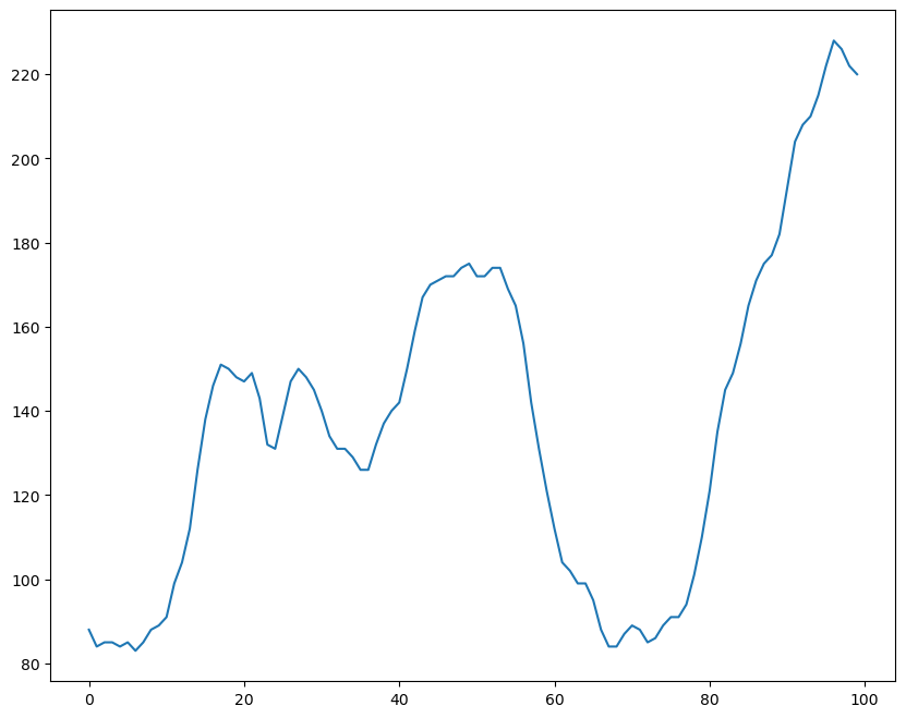
fig = plt.figure(figsize = (10, 8))
ax = fig.add_subplot(1,1,1)
ax.plot(df['value'])
plt.show()
Total samples are: 100
ARIMA(p,d,q)#
p: order of autocorrection
d: order of differential
q: order of moving average
The key to build a ARIMA model is to choose proper p, d, q
from statsmodels.graphics.tsaplots import plot_acf, plot_pacf

plot_acf(df.value)
plt.show()
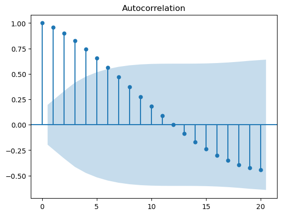
Clearly, the data is not ideal for the ARIMA model to directly start autoregressive training. So let’s see how the differencing segment of ARIMA makes the data stationary.
f = plt.figure(figsize = (12, 5))
ax1 = f.add_subplot(121)
ax1.set_title("1st order differencing")
ax1.plot(df.value.diff())

ax2 = f.add_subplot(122)
plot_acf(df.value.diff().dropna(),ax=ax2)
plt.show()
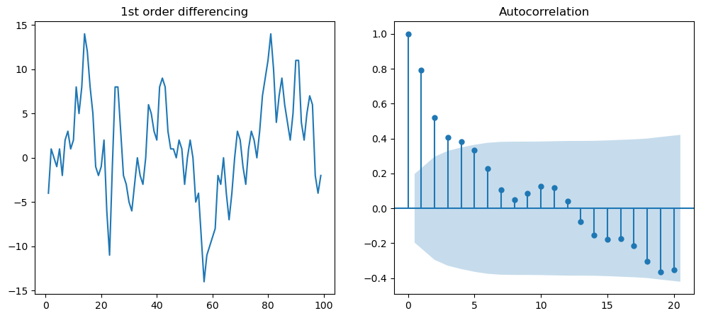
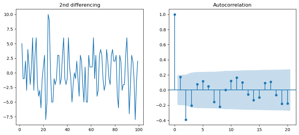
As seen above, first-order differencing shakes up autocorrelation considerably. We can also try 2nd order differencing to enhance the stationary nature.
# In the following, we will do for second differencing
f = plt.figure(figsize = (12, 5))
ax1 = f.add_subplot(121)
ax1.set_title('2nd differencing')
ax1.plot(df.value.diff().diff())

ax2 = f.add_subplot(122)
plot_acf(df.value.diff().diff().dropna(),ax=ax2)
plt.show()
# Non stationary test by ADF test

from statsmodels.tsa.stattools import adfuller
result = adfuller(df.value.dropna())
print('p-value: ', result[1])

result = adfuller(df.value.diff().dropna())
print('p-value: ', result[1])

result = adfuller(df.value.diff().diff().dropna())
print('p-value: ', result[1])
p-value:  0.12441935447109487
p-value:  0.07026846015272728
p-value:  2.843428755547158e-17
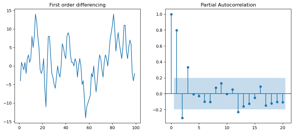
# Next we can determine the value of "p" for first differencing
f = plt.figure(figsize=(12,5))
ax1 = f.add_subplot(121)
ax1.set_title('First order differencing')
ax1.plot(df.value.diff().dropna())

ax2 = f.add_subplot(122)
plot_pacf(df.value.diff().dropna(), ax=ax2)
plt.show()
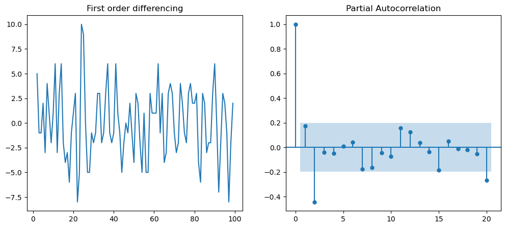
# Next we can determine the value of "p" for second differencing
f = plt.figure(figsize=(12,5))
ax1 = f.add_subplot(121)
ax1.set_title('First order differencing')
ax1.plot(df.value.diff().diff().dropna())

ax2 = f.add_subplot(122)
plot_pacf(df.value.diff().diff().dropna(), ax=ax2)
plt.show()
Thus, final ARIMA model defined as ARIMA(p=1, d=1,q= 2).#
PART II: Fit the ARIMA model#
from statsmodels.tsa.arima.model import ARIMA

arima_model = ARIMA(df.value, order = (1,1,2))
model = arima_model.fit()
print(model.summary())
                               SARIMAX Results
==============================================================================
Dep. Variable:                  value   No. Observations:                  100
Model:                 ARIMA(1, 1, 2)   Log Likelihood                -254.126
Date:                Fri, 20 Jan 2023   AIC                            516.253
Time:                        18:47:18   BIC                            526.633
Sample:                             0   HQIC                           520.453
                                - 100
Covariance Type:                  opg
==============================================================================
                 coef    std err          z      P>|z|      [0.025      0.975]
------------------------------------------------------------------------------
ar.L1          0.6976      0.130      5.365      0.000       0.443       0.952
ma.L1          0.4551      0.169      2.699      0.007       0.125       0.786
ma.L2         -0.0664      0.157     -0.424      0.671      -0.373       0.241
sigma2         9.7898      1.421      6.889      0.000       7.005      12.575
===================================================================================
Ljung-Box (L1) (Q):                   0.00   Jarque-Bera (JB):                 0.09
Prob(Q):                              0.98   Prob(JB):                         0.95
Heteroskedasticity (H):               0.63   Skew:                            -0.07
Prob(H) (two-sided):                  0.19   Kurtosis:                         3.03
===================================================================================

Warnings:
[1] Covariance matrix calculated using the outer product of gradients (complex-step).
# test another setting of (p, d,q)

arima_model = ARIMA(df.value, order = (1,2,2))
model = arima_model.fit()
print(model.summary())
                               SARIMAX Results
==============================================================================
Dep. Variable:                  value   No. Observations:                  100
Model:                 ARIMA(1, 2, 2)   Log Likelihood                -252.594
Date:                Fri, 20 Jan 2023   AIC                            513.189
Time:                        18:48:28   BIC                            523.529
Sample:                             0   HQIC                           517.371
                                - 100
Covariance Type:                  opg
==============================================================================
                 coef    std err          z      P>|z|      [0.025      0.975]
------------------------------------------------------------------------------
ar.L1          0.6530      0.103      6.359      0.000       0.452       0.854
ma.L1         -0.4743      2.191     -0.217      0.829      -4.768       3.819
ma.L2         -0.5251      1.130     -0.465      0.642      -2.740       1.689
sigma2         9.8299     21.283      0.462      0.644     -31.884      51.544
===================================================================================
Ljung-Box (L1) (Q):                   0.00   Jarque-Bera (JB):                 0.22
Prob(Q):                              0.95   Prob(JB):                         0.90
Heteroskedasticity (H):               0.61   Skew:                            -0.11
Prob(H) (two-sided):                  0.16   Kurtosis:                         3.08
===================================================================================

Warnings:
[1] Covariance matrix calculated using the outer product of gradients (complex-step).
model.plot_predict(dynamic=False)
plt.show()
---------------------------------------------------------------------------
AttributeError                            Traceback (most recent call last)
~\AppData\Local\Temp\ipykernel_26020\2666529794.py in <cell line: 1>()
----> 1 model.plot_predict(dynamic=False)
      2 plt.show()

~\Anaconda3\lib\site-packages\statsmodels\base\wrapper.py in __getattribute__(self, attr)
     32             pass
     33
---> 34         obj = getattr(results, attr)
     35         data = results.model.data
     36         how = self._wrap_attrs.get(attr)

AttributeError: 'ARIMAResults' object has no attribute 'plot_predict'
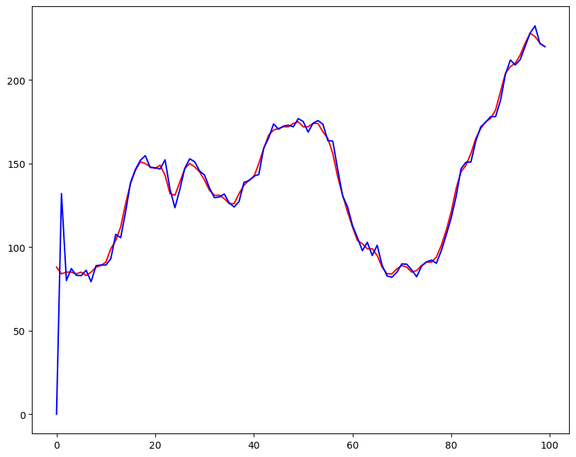
plt.figure(figsize = (10,8))
plt.plot(df.value, color = 'r')
plt.plot(model.predict(),color = 'b')
plt.show()
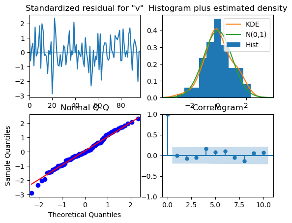
model.plot_diagnostics()